Comparing Kalman Filter with Recurrent-based machine learning on Satellite Attitude Determination

Problem Statement

Satellite Attitude Determination and Control System (ADCS) is an essential component for almost every satellite mission. It provides the satellite in-suite velocity and orientation information. However, we do not have enough ground station to track every satellite in the sky. Therefore, we need to develop an onboard system to estimate the satellite’s attitude. The widely used method is the Kalman Filter or its upgraded version, the Extended Kalman Filter. However, the Kalman Filter is not suitable for nonlinear systems. Therefore, we need to develop a new method to estimate the satellite’s attitude. The goal of this project is to compare the Kalman Filter with Recurrent-based machine learning (Bi-GRU) on Satellite Attitude Determination.

Kalman Filter (KF)

The Kalman Filter is an algorithm that uses a series of measurements observed over time, containing statistical noise and other inaccuracies, and produces estimates of unknown variables that tend to be more accurate than those based on a single measurement alone. KF is a recursive algorithm that estimates the state of a linear dynamic system from a series of noisy measurements.

Derivation of Kalman Filter

KF is derived from the following assumptions:

The state transition matrix $A$ and the observation matrix $H$ are linear.
The process noise $Q$ and the observation noise $R$ are Gaussian white noise.
The initial state $x_{0}$ and the initial state covariance $P_{0}$ are known.
The control input $u_{k}$ is known.
The observation vector $z_{k}$ is known.

where $x_{k}$ is the state vector, $A$ is the state transition matrix, $B$ is the control input matrix, $u_{k}$ is the control input, $P_{k}$ is the state covariance matrix, $Q$ is the process noise covariance matrix, $K_{k}$ is the Kalman Gain, $H$ is the observation matrix, $R$ is the observation noise covariance matrix, and $z_{k}$ is the observation vector, then derived from the following steps:

Predict: Predict the state vector $\hat{x}_{k}$ and the state covariance matrix $P_{k}$ using the state transition matrix $A$, the control input matrix $B$, the control input $u_{k}$, the state covariance matrix $P_{k-1}$, and the process noise covariance matrix $Q$.

Update: Update the state vector $\hat{x}_{k}$ and the state covariance matrix $P_{k}$ using the Kalman Gain $K_{k}$, the observation matrix $H$, the observation noise covariance matrix $R$, the observation vector $z_{k}$, and the state vector $\hat{x}_{k}$.

The following mathematical equations show how the Golden Rules of KF works:

\[\begin{aligned} \text{Predict:} \quad & \hat{x}_{k} = A \hat{x}_{k-1} + B u_{k} \\ & P_{k} = A P_{k-1} A^{T} + Q \\ & \\ \text{Update:} \quad & K_{k} = P_{k} H^{T} (H P_{k} H^{T} + R)^{-1} \\ & \hat{x}_{k} = \hat{x}_{k} + K_{k}\left(z_{k} - H \hat{x}_{k}\right) \\ & P_{k} = (I - K_{k} H) P_{k} \end{aligned}\]

It is an optimal estimator that minimizes the mean squared error of the estimated state vector $\hat{x}_{k}$.

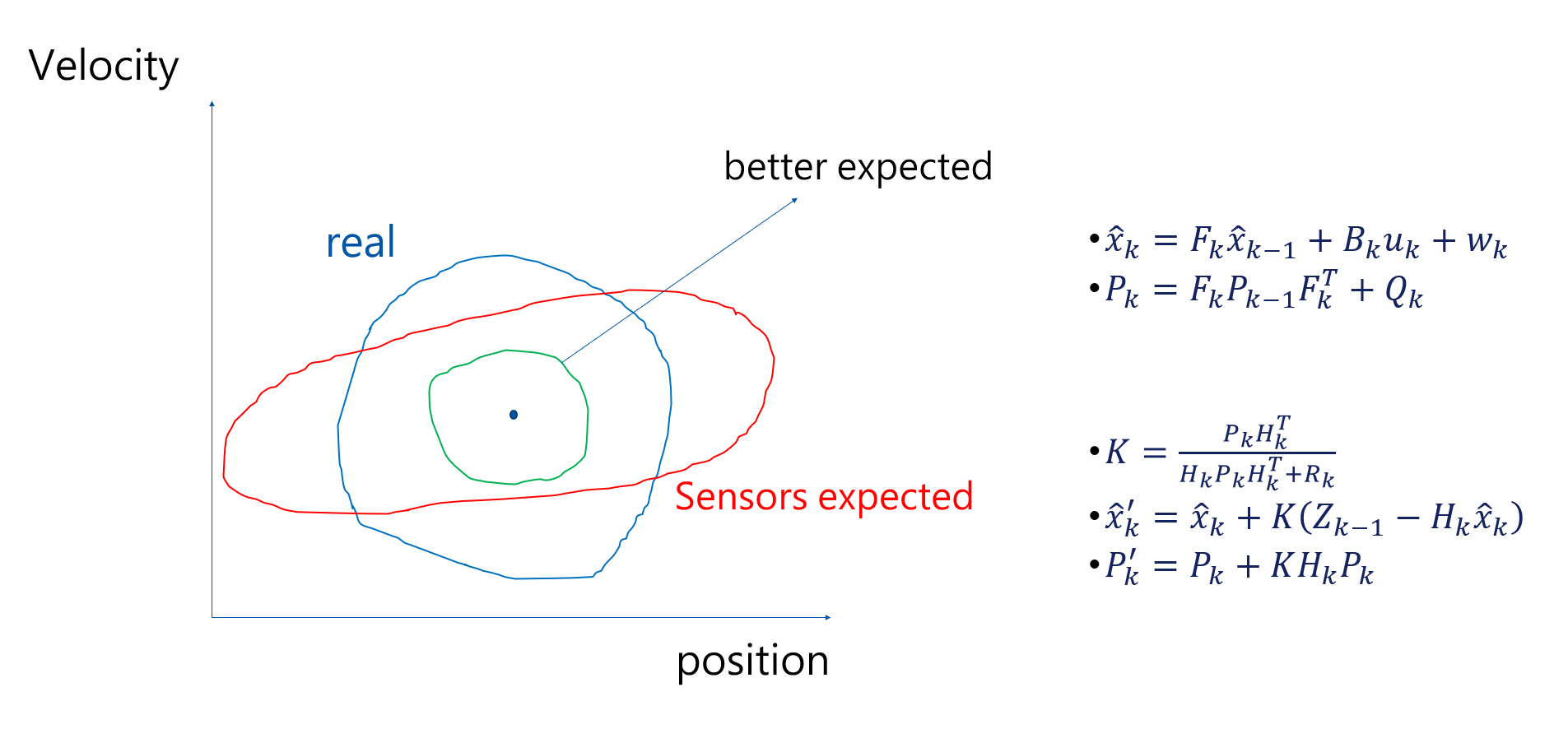
Iillustration of how Kalman Filter works

Recurrent-based machine learning (Bi-GRU)

The Recurrent-based machine learning (Bi-GRU) is a type of neural network that is suitable for sequential data. It is a type of Recurrent Neural Network (RNN) that is capable of learning long-term dependencies with following configuration : [Forward GRU, Backward GRU]. The following mathematical equations show how the Bi-GRU works:

\[\begin{aligned} \text{Forward GRU:} \quad & z_{t} = \sigma\left(W_{z} x_{t} + U_{z} h_{t-1} + b_{z}\right) \\ & r_{t} = \sigma\left(W_{r} x_{t} + U_{r} h_{t-1} + b_{r}\right) \\ & \tilde{h}_{t} = \tanh\left(W h_{t-1} + U\left(r_{t} \odot x_{t}\right) + b\right) \\ & h_{t} = z_{t} \odot h_{t-1} + (1 - z_{t}) \odot \tilde{h}_{t} \\ & \\ \text{Backward GRU:} \quad & z_{t} = \sigma\left(W_{z} x_{t} + U_{z} h_{t+1} + b_{z}\right) \\ & r_{t} = \sigma\left(W_{r} x_{t} + U_{r} h_{t+1} + b_{r}\right) \\ & \tilde{h}_{t} = \tanh\left(W h_{t+1} + U\left(r_{t} \odot x_{t}\right) + b\right) \\ & h_{t} = z_{t} \odot h_{t+1} + (1 - z_{t}) \odot \tilde{h}_{t} \end{aligned}\]

where $x_{t}$ is the input vector at time $t$, $h_{t}$ is the hidden state vector at time $t$, $W_{z}$, $U_{z}$, $b_{z}$, $W_{r}$, $U_{r}$, $b_{r}$, $W$, $U$, $b$ are the weight matrices and bias vectors, $\sigma$ is the sigmoid activation function, $\tanh$ is the hyperbolic tangent activation function, and $\odot$ is the element-wise multiplication.

Dataset

The dataset used for this project is credited to the 3U CubeSat - (IDEASSat/INSPIRESat-2), which saved its ADCS data in ECEF (Earth-Centered, Earth-Fixed) coordinate system in every 30 seconds. However, due to single particle event and minor hardware failure, the data is not continuous. Therefore, we concatenate the data from different days to form a continuous dataset (since it will pass by the same ground station every day, we can observe from the data that it does have some periodicity after we drop the data with single particle event).

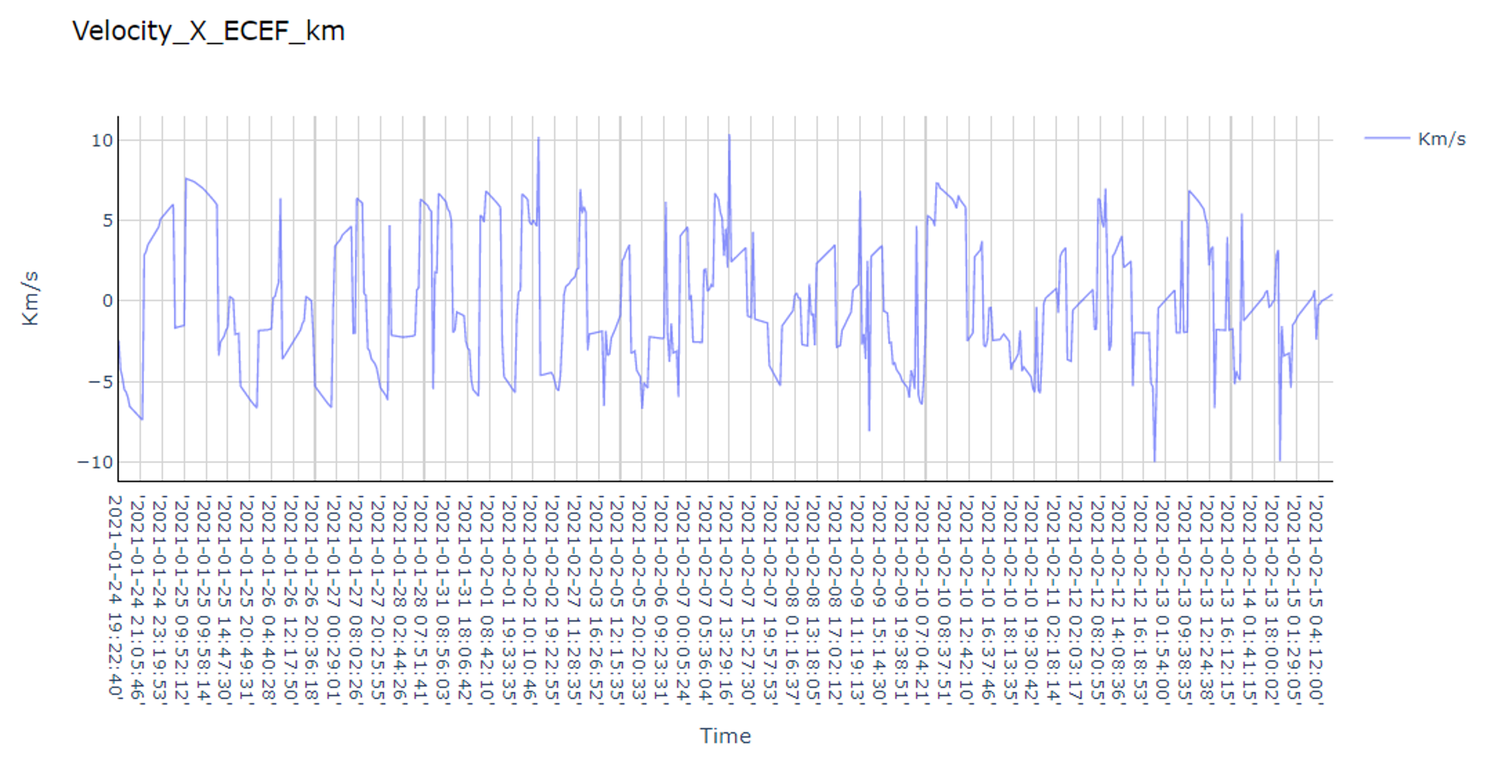
Concate the data from different days

In addition, we also use the System Tool Kit (STK) to simulate the IDEASSat in the ECEF coordinate system. The following image shows the ECEF Velocity - Xaxis of the IDEASSat simulated by STK with the same time period as the dataset.

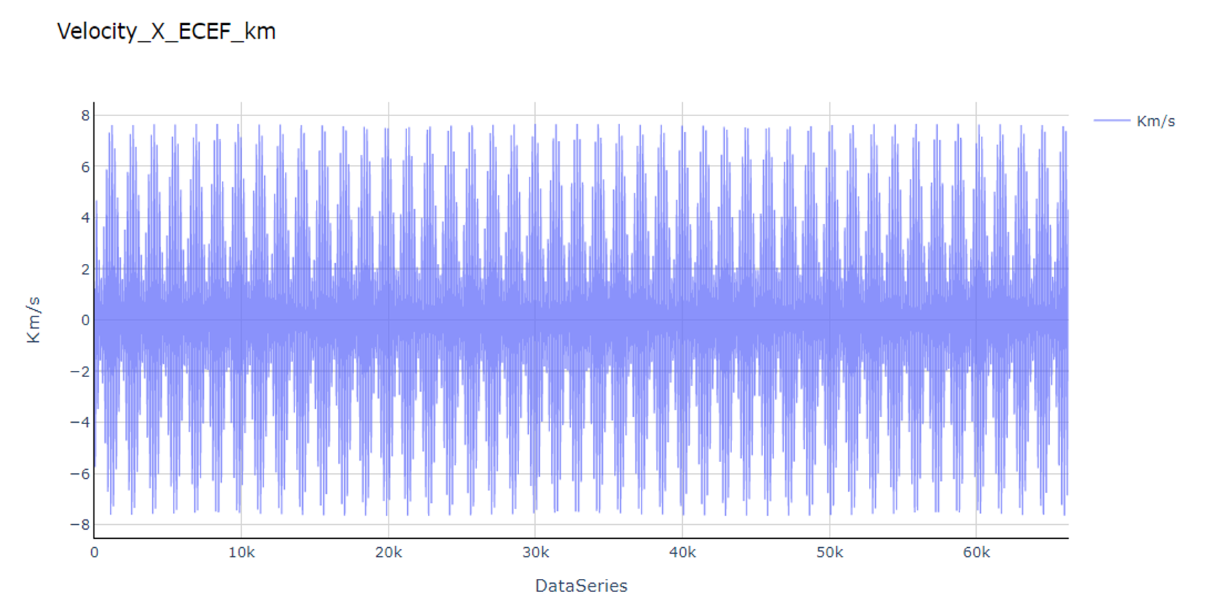
System Tool Kit simulation of IDEASSat

Results

The following results show the comparison between the Kalman Filter and Bi-GRU on the ECEF Velocity - Xaxis of the IDEASSat.

Kalman Filter

Position and Velocity: Estimate the satellite’s initial position $x_0$ and velocity $\dot{x}_0$.
$P_0$: A diagonal covariance matrix representing the error in the initial state estimate.
$Q$: Reflects uncertainty in the model predictions, to be estimated based on actual conditions.
$R$: Represents noise and uncertainty in measurements, such as radar measurement errors.
$A$: Describes how the state (position and velocity) transitions from one time step to the next.
$H$: Matrix used to transform state variables into observable quantities. In this case, it is the identity matrix.

Bi-GRU

Features: ECEF Coordinate - Xaxis, ECEF Coordinate - Yaxis, ECEF Coordinate - Zaxis, ECEF Acceleration - Xaxis, ECEF Acceleration - Yaxis, ECEF Acceleration - Zaxis
Target: ECEF Velocity - Xaxis

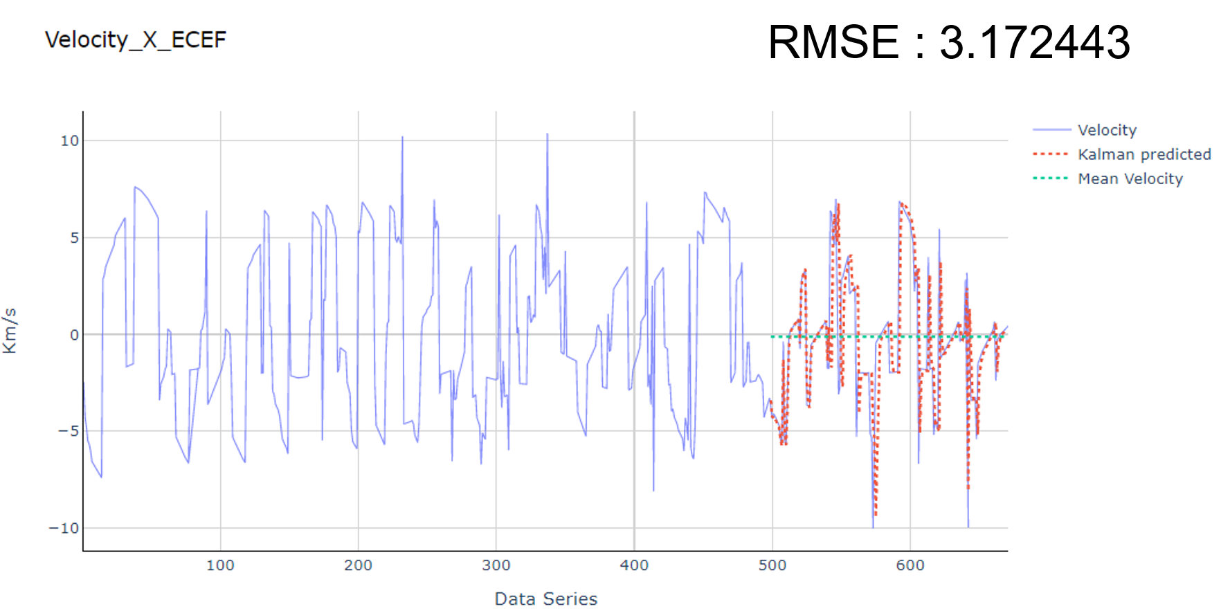
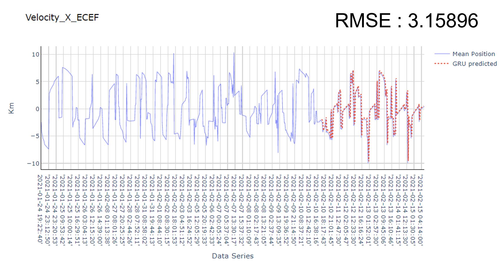
Comparison between Kalman Filter and Bi-GRU on ECEF Velocity - Xaxis of the IDEASSat

Upper: Kalman Filter, Lower: Bi-GRU

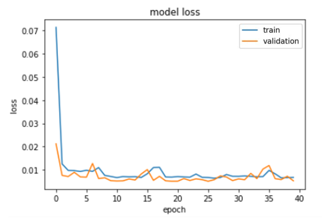
Loss graph of Bi-GRU

I also implemented the same Bi-GRU model on the STK simulated data. Showing that the Bi-GRU can well capture the periodicity of the IDEASSat.

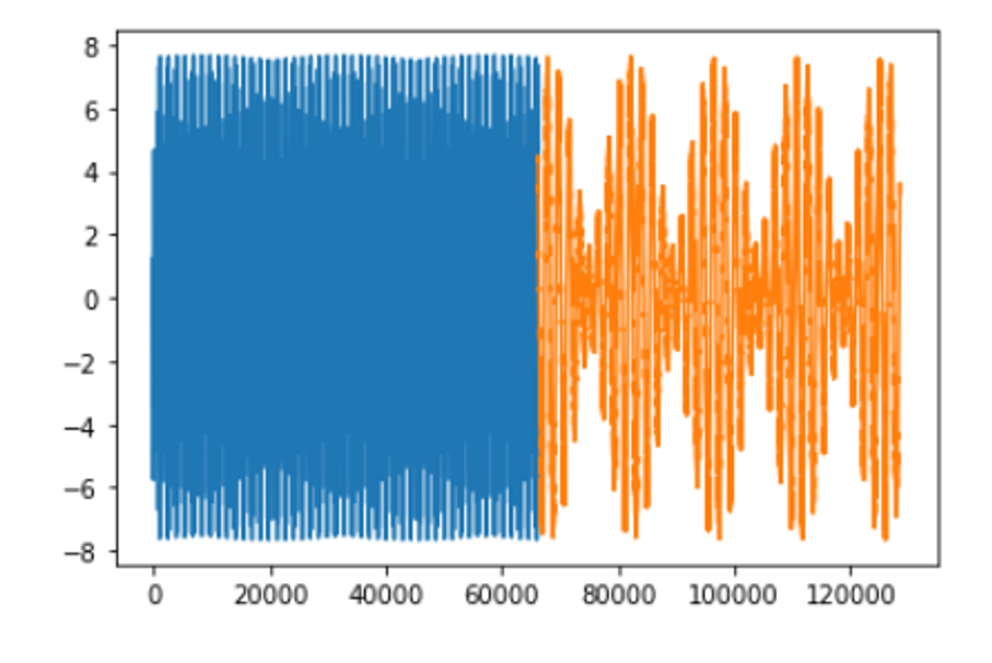
Bi-GRU on STK simulated data

Conclusion

In this project, we discuss the derivation of the Kalman Filter and the Bi-GRU. We also compare the Kalman Filter with the Bi-GRU on the ECEF Velocity - Xaxis of the IDEASSat. The results show that the Bi-GRU can well capture the periodicity of the IDEASSat. However, it only slightly competes with the Kalman Filter on this non-linear system, which means that it may not outperform the Extended Kalman Filter. There are several studies that show Recurrent-based machine learning can outperform the Kalman Filter on the non-linear system. Therefore, we need to further investigate the Bi-GRU on the non-linear system to see if it can outperform the Kalman Filter, or the more important, obtain more consistent and continuous dataset to improve the performance of the Bi-GRU.

References

Zhou, M., Xu, G., Li, X., & Wang, Y. (2021). Title of the Article. Remote Sensing, 13(6), 1185. https://doi.org/10.3390/rs13061185
Li, X. R., & Jilkov, V. P. (2000). Survey of maneuvering target tracking: Dynamic models. In O. E. Drummond (Ed.), Proceedings of SPIE (Vol. 4048, pp. 212-235). https://doi.org/10.1117/12.391979
MATLAB Linear Kalman Filter. (n.d.). Retrieved from https://www.mathworks.com/help/fusion/ug/linear-kalman-filters.html
Meng, S., Jiang, X.Q., Gao, Y., Hai, H. (2020). Performance evaluation of channel decoder based on recurrent neural network. Journal of Physics: Conference Series, 1438(1), 012001. https://doi.org/10.1088/1742-6596/1438/1/012001